When studying vibration mechanics, beams are one of the most fundamental and practical examples of multi-degree-of-freedom systems.
Even though real-world equipment can be complex, most vibration problems can be approximated using beam models.
In this article, we’ll break down the equation of motion for a vibrating beam, explain how it connects to the simpler single-degree system, and show how material mechanics concepts (like bending moment and deflection) are applied in vibration analysis.
Whether you’re a student or an engineer refreshing your knowledge, this guide focuses on understanding rather than lengthy derivations.
1. The Beam Vibration Model
A vibrating beam represents a continuous system with many degrees of freedom.
While a one-degree-of-freedom model describes a simple mass-spring motion, a beam allows deflection along its length.
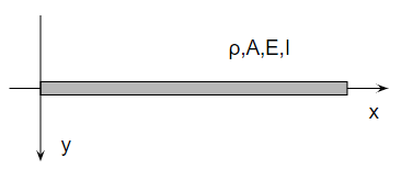
Key parameters:
- ρ : Density (kg/m³)
- A : Cross-sectional area (m²)
- E : Young’s modulus (N/mm²)
- I : Second moment of area (mm⁴)
Among these, ρ and E are determined by material selection, while A and I depend on geometry.
2. Relationship Between Deflection, Slope, and Moment
In material mechanics, the following relationships hold for a beam along the x-axis:
| Quantity | Symbol | Definition |
|---|---|---|
| Deflection | y | Displacement at position x and time t → y(x,t) |
| Slope | Θ | dy/dx |
| Moment | M | –EI (d²y/dx²) |
| Shear force | N | dM/dx |
These relationships are the foundation for developing the beam’s motion equation.
3. The Equation of Motion
The differential equation governing beam vibrations is:
$$ ρA\frac{\partial^2 y(x,t) }{\partial t^2 }+EI\frac{\partial^4 y(x,t) }{\partial x^4 } = f(x,t) $$
This is analogous to the one-degree vibration model:
$$ m\ddot{x}+kx=f $$
- The first term (ρA) represents mass and inertia.
- The second term (EI) represents restoring force (elastic stiffness).
- The right-hand side f(x,t) represents external force.
Each segment of length dx carries a small mass (ρA dx) and is affected by shear and bending moments, producing internal restoring forces.
4. Natural Frequency and Mode Shapes
To find the natural frequencies, we use the method of separation of variables:
$$ y(x,t)=φ(x)ψ(t) $$
Substituting into the motion equation gives:
$$ ρAφ(x)\frac{\partial^2 ψ(t)}{\partial t^2 }+EIψ(t)\frac{\partial^4 φ(x) }{\partial x^4 } = 0 $$
This separates into two independent equations:
Time-dependent part:
$$ \frac{1}{ψ(t)}\frac{\partial^2 ψ(t)}{\partial t^2 } = C $$
whose solution is
$$ ψ(t)=Ae^{iωt} $$
where ω is the natural frequency.
Spatial part:
$$ -\frac{ρA}{EI}\frac{1}{φ(x)}\frac{\partial^4 φ(x) }{\partial x^4 } = C $$
The general solution is:
$$ φ(x)=B_1sin(λx)+B_2cos(λx)+B_3sinh(λx)+B_4cosh(λx) $$
Boundary conditions (fixed or free ends) determine λ and ω.
Each solution corresponds to a mode shape, and a real beam’s vibration is a combination of these modes — similar to a Fourier series.
5. Practical Notes
Analytical solutions quickly become complex, so engineers often rely on numerical methods such as MATLAB, ANSYS, or other FEM tools.
However, understanding this fundamental equation is crucial for interpreting simulation results or identifying unrealistic outputs.
Conclusion
The beam vibration equation forms the basis of advanced vibration analysis.
It connects material mechanics with dynamic systems and provides insight into how real structures behave under oscillating forces.
Even though the math can be heavy, remembering that it’s just an extension of the single-degree-of-freedom system helps you keep perspective.
About the Author – NEONEEET
A user‑side chemical plant engineer with 20+ years of end‑to‑end experience across design → production → maintenance → corporate planning. Sharing practical, experience‑based knowledge from real batch‑plant operations. → View full profile
Comments