In vibration engineering, the equation of motion for a cantilever beam is one of the most fundamental models.
However, when we want to make the model more realistic — closer to actual mechanical systems — we need to increase the degrees of freedom.
This article explains how to derive and interpret the equation of motion for a beam with an attached point mass and spring.
Understanding this concept is essential before performing numerical analysis, since physical intuition supports correct model verification.
This article is part of our vibration analysis series:
- Overview of Single-Degree-of-Freedom Vibration Systems
- Fundamentals of Two-Degree-of-Freedom Systems
- Equation of Motion for Beam Vibrations Explained Simply
- Influence of Equipment Vibrations on Beams and Foundations
1. Basic Equation of Motion
Let’s start with the beam alone.
The standard equation of motion for a uniform beam is:
$$ ρA\frac{\partial^2 y(x,t) }{\partial t^2 }+EI\frac{\partial^4 y(x,t) }{\partial x^4 } = f(x,t) $$
Now, we attach a point mass at position xm, connected by a spring with stiffness k.
The equations become:
$$ ρA\frac{\partial^2 y(x,t) }{\partial t^2 }+EI\frac{\partial^4 y(x,t) }{\partial x^4 } = k(y_m(t)-y(x_m,t)) $$
$$ m\frac{\partial^2 y_m(t) }{\partial t^2 } = -k(y_m(t)-y(x_m,t)) $$
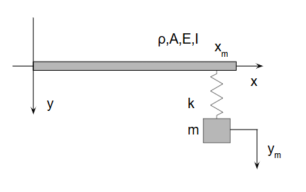
Here, y(xm,t) is the beam displacement at xm, and ym(t) is the displacement of the attached mass.
2. Combined Equation
By adding both equations, the spring forces cancel:
$$ ρA\frac{\partial^2 y(x,t) }{\partial t^2 }+EI\frac{\partial^4 y(x,t) }{\partial x^4 }+m\frac{\partial^2 y_m(t) }{\partial t^2 } = 0 $$
Although the beam is a continuous system, in numerical modeling we typically treat it as discrete nodes, so we can express displacements as:
$$ \mathbf{y(x,t)}=\begin{pmatrix} y_{1}(t) \\ \dots \\ y_{n}(t) \end{pmatrix} $$
By applying mode separation (modal analysis), we can write:
$$ \mathbf{y(x,t)}=\begin{pmatrix} ψ_{11} & ψ_{12} & \dots & ψ_{1n} \\ \dots \\ ψ_{n1} & ψ_{n2} & \dots & ψ_{nn} & \end{pmatrix} \begin{pmatrix} φ_{1}(t) \\ \dots \\ φ_{n}(t) \end{pmatrix}$$
When including the mass, the system becomes n+1n + 1n+1 degrees of freedom:
$$ \mathbf{y'(x,t)}=\begin{pmatrix} y_{1}(t) \\ \dots \\ y_{n}(t) \\ \color{red}{y_{m}(t)} \end{pmatrix} $$
This structure shows how the added mass changes the dynamic mode shapes of the beam.
3. Parameter Considerations
Let’s interpret how the system changes when parameters vary.
Case 1: m=0
If there’s no attached mass, the last row disappears, and the system reduces to the standard beam model.
This confirms our model’s consistency.
Case 2: m=∞
If the attached point is fixed (infinite mass), it behaves like a clamped end condition.
For a free end (node nnn), we can express it as:
$$ \mathbf{y'(x,t)}=\begin{pmatrix} ψ_{11} & ψ_{12} & \dots & ψ_{1n} & ψ_{1m}\\ \dots \\ ψ_{n1} & ψ_{n2} & \dots & ψ_{nn} & ψ_{nm} \\ψ_{m1} & ψ_{m2} & \dots & ψ_{mn}& m/ρAψ_{mm} \end{pmatrix} \begin{pmatrix} φ_{1}(t) \\ \dots \\ φ_{n}(t) \\ \color{red}{φ_{m}(t)} \end{pmatrix}$$
As m→∞, the last row becomes meaningless, reducing the degrees of freedom accordingly.
Regardless of position, the added mass alters the eigenmodes — a natural outcome of the beam’s dynamic interaction.
4. Interpretation
The key takeaway is that adding a point mass introduces coupling effects between adjacent nodes, changing the natural frequencies and mode shapes.
Understanding these effects helps in developing more accurate dynamic models for mechanical structures, such as plant equipment, rotors, and piping systems.
Conclusion
A beam with an attached mass and spring extends the simple cantilever model into a more realistic representation of actual structures.
By comparing different mass conditions — m=0m=0m=0, m=∞m=∞m=∞ — you can clearly see how boundary conditions and local stiffness affect vibration behavior.
Mastering this concept bridges the gap between theoretical vibration models and real-world simulation results.
Comments